Othogonal Calculators
Orthogonals explained.
 Consider a continuous curve (path) in 2D space, at any point along the curve there
is a
single tangent line and two normals (orthogonals).
Consider a continuous curve (path) in 2D space, at any point along the curve there
is a
single tangent line and two normals (orthogonals).
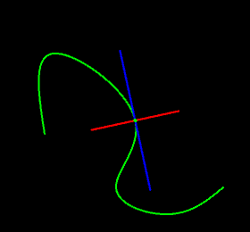
This picture shows the tangent line (blue) and the 2 orthogonals (red) for a single point on the curve (green).
It might look like there is just one orthogonal but in fact there are two, one on each side of the line. They look like one because there is 180° angle between them.
In 2D graphic applicatione we could use the tangent or the orthogonal to align a shape to the curve.
 In 3D
space it is slightly more complicated, although there is a
single tangent at any point along the curve there are an infinite
number of orthogonals.
In 3D
space it is slightly more complicated, although there is a
single tangent at any point along the curve there are an infinite
number of orthogonals.
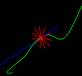
In this picture there is a continuous curve (path) shown in green, as before we have a sibgle tangent line (blue) but now the orthogonal to the curve is not a line but a 2D plane. This means there are an infinite number of orthogonals, the picture shows just a few of them in red.
To align a shape to the curve both the tangent and the orthogonal are required but with an infinite number to choose from how to pick the best orthogonal and does it matter.
A bad choice of orthogonal can cause unwanted rotations and / or twists in the cross-section. Shapes3D will choose what it believes to be the best orthononal calculator from four different algorithms but if it doesn't work the user can specify the calculator to use when creating the path. The choices are
|
|
|
|
If this doesn't work the user can create their own orthogonal calculator class and use that.